Predator-Prey

During the covid pandemic I’ve been learning about dynamic systems in biology from a textbook, Modeling Life^[1]. To go deeper into the math I’ve been watching Robert Ghrist’s lectures^[2]. To go deeper into the biology I’ve been watching the MIT Systems Biology class^[3]. I haven’t yet read Physical Models of Living Systems^[4].

One of the early 2-variable examples is the predator-prey model (“Lotka Volterra”). I’m not doing all the homeworks but instead I wanted to pick a handful of projects to dive into, and I decided this would be the first.

These were originally rough notes that I polished over time as I learned the material. See my blog post^[5] to see how earlier versions of this page looked.

 1  Lotka-Volterra#

The main idea is that there’s a prey animal \(x\) 🐇 and a predator animal \(y\) 🦊. When the prey population increases, it provides more food for predators to multiply.

The Lotka-Volterra rules are:

1. Birth: the prey increases on its own: \(+α \cdot x\)
2. Malnourishment: the predators decrease on their own: \(-γ \cdot y\)
3. Predation: the prey decreases due to predators: \(-β \cdot x \cdot y\)
4. Predation: the predators increase due to prey: \(+δ \cdot x \cdot y\)

These rules aren’t a particularly good model but they’re simple. This model is widely studied and seems like a good starting point for me to learn this type of system. It also has some surprising behavior that I want to explore in the simulations. The rules give us these differential equations which could be implemented in code:

dx_dt = alpha*x - beta*x*y
dy_dt = delta*x*y - gamma*y

x += dx_dt * dt
y += dy_dt * dt

The chart above shows the populations over time. You can see they’re repeating. There’s a different type of chart, the phase diagram^[6], which plots the two populations together but without time:

This shows how the two variables related, but not how fast they’re moving. Both of these 2d diagrams are views of a 3d diagram (time, predator, prey), which might be fun to make but I didn’t get around to doing so. It’d look like this:

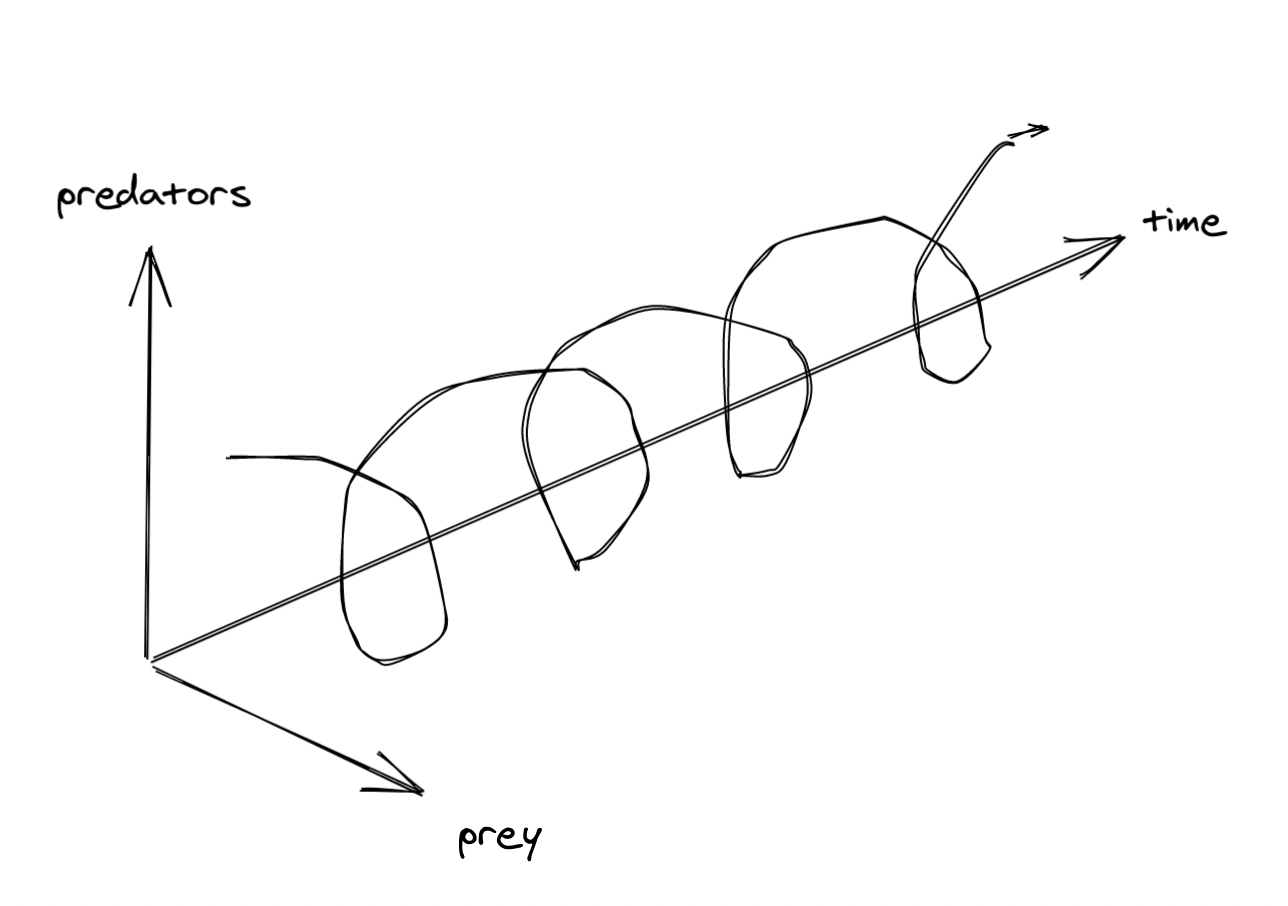
Viewed from the side or top, it’s a plot of predators or prey over time. But viewed from the end, it’s a phase plot. It’d be a cool animation but it’s a bit of work so I didn’t make it. I did read a little bit about how to draw vector (this paper^[7] and this blog post)^[8] and I experimented a little bit^[9].

What else can I explore?

 1.1. Period#

The period of the cycle is how long it takes before it repeats. The Wikipedia page^[10] says the period is \(2π / \sqrt{\color{#00a}α \color{#a44}γ}\). For my default values of \(\textcolor{#00a}{α} = \frac{2}{3}, \textcolor{#a44}{γ} = 1\), that means the period is around 7.695 seconds. But my numerical integration doesn’t produce that! It’s not even close. It turns out that the formula only applies at the equilibrium point, and I didn’t find a formula at any other point.

Would it be interesting to display the period for every set of parameters?

{ need to try it and see }

{My implementation is fast enough that I can calculate period, min, max, mean and then do something with it, like plot them for many parameter values at a time. “Ladder of abstraction”. Since there are cycles, I need to map each point to a cycle, and then I can plot the cycle vs the period/min/max/mean. I could use the max as the cycle number, and then I’d be plotting period/min/mean vs max? Alternatively I could use a 2d input with starting }

 1.2. Equilibrium#

The equilibrium point is when the population stays the same.

• prey \(x = \frac{\color{#a44} γ}{\color{#a44} δ}\)
• predators \(y = \frac{\color{#00a} α}{\color{#00a} β}\)

When I compare this to the equations

\[\begin{aligned} \frac{dx}{dt} & = \textcolor{#00a}{\alpha} x - \textcolor{#00a}{\beta} x y \\ \frac{dy}{dt} & = \textcolor{#a44}{\delta} x y - \textcolor{#a44}{\gamma} y \end{aligned}\]

I was a bit surprised that the equilibrium for predators \(y\) depends only on the parameters in the prey equation \(\frac{dx}{dt}\), and the equilibrium for prey \(x\) depends only on the parameters in the predator equation \(\frac{dy}{dt}\).

• \(\color{#00a} α\): prey birth rate
• \(\color{#00a} β\): proportional of prey eaten by predators
• \(\color{#a44} γ\): death rate of malnourished predators
• \(\color{#a44} δ\): number of predator born per 1 prey eaten

I would expect that the equilbrium for prey would depend on the prey birth rate, \(\color{#00a} α\), but it doesn’t! And the equilibrium for predators does not depend on the death rate of predators. This both means the model can be surprising (good for math!), and that the model likely does not match reality (bad for biology!).

There’s also an equilibrium point when both predator and prey are at 0, but that’s not so interesting.

 1.3. Mean, min, max#

The mean should be the average value over one cycle. I don’t see this mentioned on the Wikipedia page or the textbook.

But I discovered by calculating and plotting the mean that it’s equal to the equilibrium!

Similarly, I can calculate the min and max numerically but I don’t see an analytical way to calculate this.

 1.4. Intervention#

One of the more fascinating things I read in the Modeling Life textbook is that there’s counterintuitive behavior when intervening in the population:

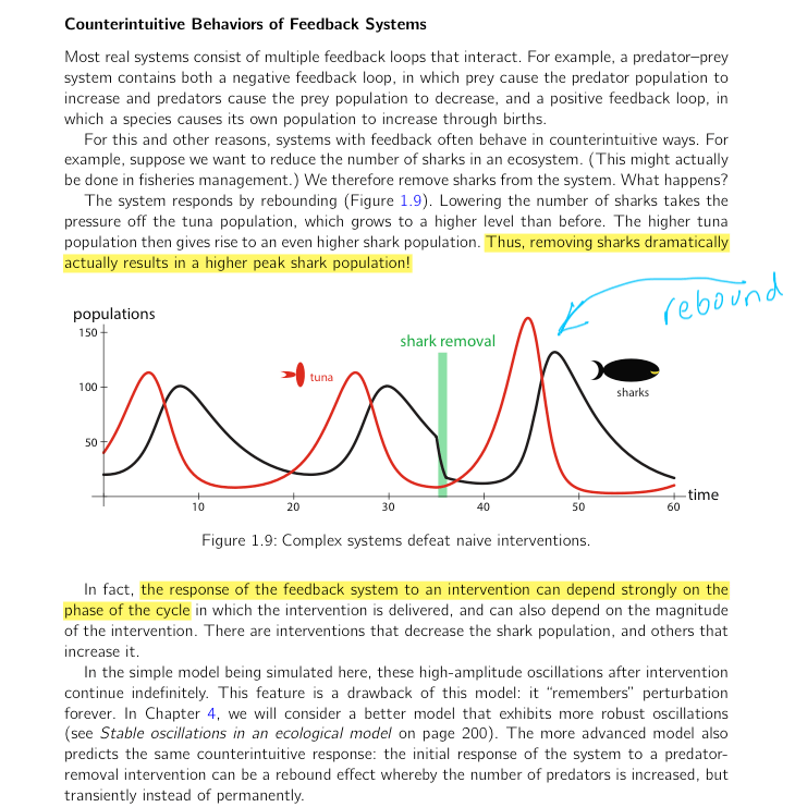
Reducing the predator population can cause the predator population to go up higher than it had been. The textbook says that it depends on which phase of the cycle you’re in when you reduce the population. I wanted to see for myself, so I wrote the simulation:

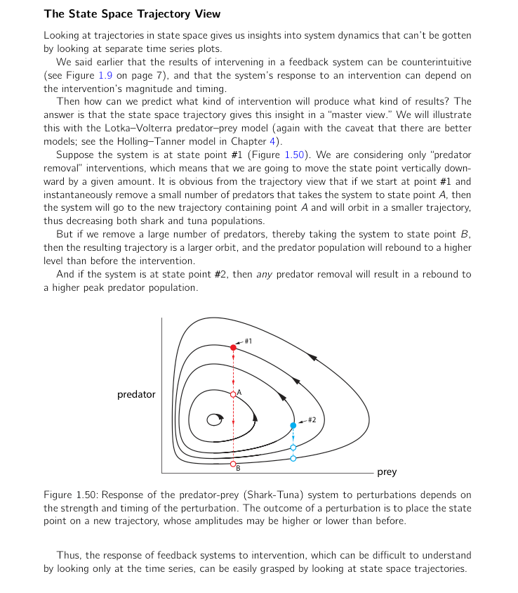
Try this: click/drag in the middle and set the predator (red) population. Try it near the bottom and the top of the cycle. See what happens to the predators and also the prey (blue). Fascinating!

Reducing the predator population slightly can either increase or decrease the maximum predator population, but reducing it by a large amount almost always increases the amount of predators! Is there a way to know when the population will decrease vs increase? At the time I wrote this page, I hadn’t gotten to that part of the book yet, but the answer is yes:

 1.5. Implementation

I used numerical integration and placed the results into Javascript typed arrays. This calculation turned out to be just as fast in the browser (Javascript, no type declarations) as in C++ or Rust (native code, type declarations, optimizing compiler). That was a bit of a surprise to me.

I had thought I should put the calculation in Web Workers so that it doesn’t interrupt the main flow of the page but I never got around to it.

I wrote some notes about accuracy of numerical integration and about the performance of various implementations I tried.

 2  Other models#

• - more sophisticated models

  • https://en.wikipedia.org/wiki/Arditi%E2%80%93Ginzburg_equations^[11]
  • https://en.wikipedia.org/wiki/Nicholson%E2%80%93Bailey_model^[12]
  • one species with an environment limit (logistic equation)
  • two competing species (lotka-volterra: https://en.wikipedia.org/wiki/Competitive_Lotka%E2%80%93Volterra_equations^[13])
  • two prey population, one resistant to predators but grows slowly
  • three populations

other stuff?

• “Lyapunov function” is a function that can be used to prove stability of a system
  • no general form; reminds me of cs proofs of bounds of algorithms
• “sensitivity analysis” - how much does behavior depend on the parameters? example: change alpha slightly, see how much the maximum population changes, or show the range of outputs for a range of inputs like on https://strimas.com/post/lotka-volterra/^[14]
• newton’s method is a discrete sequence as opposed to these continuous sequences
• logistic equation works both as continuous and discrete
• terminal velocity
• golden ratio with continued fractions - discrete sequence

• idea from discord
  • “infinite/fixed rate resources; “protected” resources (which can’t drop below a minimum); discrete reproductive cycles (if they bury eggs, and predator can’t eat eggs, less likely to eat all the birds)”

 3  More reading#

• Wikipedia: Lotka-Volterra equations^[15]
• Mike Bostock’s wonderful interactive explanation^[16]
• https://www.petercollingridge.co.uk/blog/alife/ecosystem-simulation/basic-creature-simulation/^[17]
• https://web.archive.org/web/20170506043310/http://tuvalu.santafe.edu/~albers/teaching/dynamicsbooks.html^[18] - lots of books I could be reading, but am not
• https://mc-stan.org/users/documentation/case-studies/lotka-volterra-predator-prey.html^[19] - what if you have real data and want to fit the model to it?